Author: Hugo Chenel
Purpose: This tutorial provides a comprehensive guide for advanced bulk RNA-seq data analysis in R, using publicly available datasets and Bioconductor package DESeq2. It is designed for researchers seeking to perform high-confidence differential expression analysis and perform downstream functional enrichment.
Overview
RNA‑seq has become an indispensable tool for transcriptomic analysis. In this guide, we walk through an advanced pipeline in R that covers:
- Experimental design and data preprocessing
- Quality control
- Alignment/quantification
- Data import
- Differential expression analysis
- Downstream functional enrichment & pathway analysis
- Batch correction and cofounder adjustment
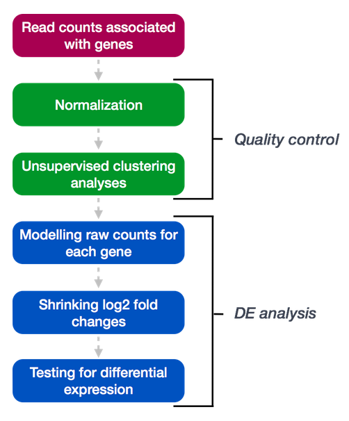
The following flowchart illustrates the general structure of the RNA-seq differential expression pipeline implemented in this tutorial. While the details will unfold step by step, this high-level view helps frame the key stages (from raw gene counts to biological insight).
1. Experimental design and data preprocessing
1.1. Experimental design considerations
Before starting any analysis, ensure your study design is robust. Consider:
- Biological replicates: Sufficient replication increases statistical power.
- Batch effects: Randomize samples across sequencing runs to minimize confounders.
- Metadata collection: Maintain detailed sample metadata (condition, batch, sex, age, …).
1.2. Data acquisition and preprocessing
Preprocessing (adapter trimming and quality filtering) is typically performed outside R using tools like FastQC, Trimmomatic or Cutadapt. Aggregate quality metrics using MultiQC.
💡 For low-level quality control in R, consider using the
ShortReadpackage from Bioconductor.
2. Alignment & quantification
2.1 Alignment vs. Pseudo-alignment
- Alignment: Tools like STAR or HISAT2 map reads to the reference genome → genome-based mapping
- Alignment/Quantification: Leverage pseudo‑alignment tools (Salmon, Kallisto) → faster transcript quantification
Use tximport to import transcript-level quantification and summarize to gene-level.
Once you have your quantification results, the next step is importing them into R.
2.2 Count matrix and metadata integration
Structure your count matrix and metadata for downstream modeling. Emphasize consistency in sample naming and use robust identifiers to link experimental conditions.
3. Library loading and data import
3.1. Load libraries
library(tximport)
library(TCGAbiolinks)
library(SummarizedExperiment)
library(DESeq2)
library(sva)
library(apeglm)
library(clusterProfiler)
library(org.Hs.eg.db)
library(ggplot2)
library(pheatmap)
3.2. Importing count data with tximport
Use the tximport package to import transcript-level quantification and summarize to the gene level. For example:
# Define paths to quantification files (from Salmon for example)
files <- list.files(path = "quant/", pattern = "quant.sf", full.names = TRUE, recursive = TRUE)
names(files) <- sub("quant/(.*)/quant.sf", "\\1", files)

# tximport expects a tx2gene mapping if txOut = FALSE
# You must include this if you're summarizing to gene-level
tx2gene <- read.csv("tx2gene.csv")  # Format: transcript_id, gene_id

# Import counts with tximport
txi <- tximport(files, type = "salmon", txOut = FALSE, tx2gene = tx2gene)

# View the imported counts
head(txi$counts)
This approach lets us work seamlessly with tools like DESeq2 (or edgeR).
3.3. Import TCGA data
We begin by querying TCGA for KICH RNA‑seq counts (STAR counts) using TCGAbiolinks. The query retrieves samples from both tumor and normal tissues.
# Query TCGA-KICH RNA-seq data for primary tumors and normals
query <- GDCquery(project = "TCGA-KICH",
                  data.category = "Transcriptome Profiling",
                  data.type = "Gene Expression Quantification",
                  workflow.type = "STAR - Counts",
                  sample.type = c("Primary Tumor", "Solid Tissue Normal"))

GDCdownload(query)
kich_data <- GDCprepare(query)

# Inspect the sample metadata to confirm sample types and batch variables if needed.
table(colData(kich_data)$sample_type) # Check distribution of tumor vs normal samples
In this tutorial, we use this publicly available RNA-seq data from TCGA-KICH, a cohort from TCGA focused on kidney chromophobe carcinoma.
More specifically, we download:
- Primary Tumor samples: representing cancerous kidney tissue
- Solid Tissue Normal samples: non-tumor kidney tissue from the same patients or population
The RNA-seq data is preprocessed using the STAR aligner, which providee gene-level raw counts. These counts are used as input for differential expression analysis with DESeq2.
Why this dataset? TCGA-KICH offers a well-annotated, real-world dataset with a clear biological contrast (tumor vs normal), making it ideal to demonstrate high-confidence RNA-seq workflows.
We also have the possibility to work with clinical metadata (like gender or smoking status) to build more complex models.
4. Differential Expression Analysis
4.1. Setup DESeq2
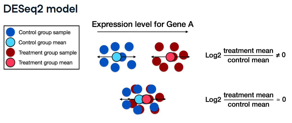
The DESeq2 model estimates gene-wise log2 fold changes by comparing the mean expression levels between groups. As shown below, if the treatment and control means differ substantially for a given gene (Gene A), a non-zero log2 fold change is observed, which indicate differential expression.
# -------------------------------
# If using tximport
# -------------------------------

# Assume 'colData' is a data frame with sample information
# and row names matching sample identifiers in txi$counts
# dds <- DESeqDataSetFromTximport(countData = txi, colData = colData, design = ~ condition + batch)

# -------------------------------
# If using TCGA
# -------------------------------

# Extract count matrix and sample metadata
count_matrix <- assay(kich_data)
sample_info <- as.data.frame(colData(kich_data))

# Ensure matching order
count_matrix <- count_matrix[, match(rownames(sample_info), colnames(count_matrix))]
stopifnot(all(rownames(sample_info) == colnames(count_matrix)))

# Create DESeq2 objects
dds <- DESeqDataSetFromMatrix(countData = count_matrix,
                              colData = sample_info,
                              design = ~ sample_type)

dds_full <- DESeqDataSetFromMatrix(countData = count_matrix,
                                   colData = sample_info,
                                   design = ~ sample_type + gender + tobacco_smoking_status)

# Filter low-count genes
dds <- dds[rowSums(counts(dds)) > 10, ]
dds_full <- dds_full[rowSums(counts(dds_full)) > 10, ]

# Relevel reference
# This ensures that differential expression results compare other groups against 'Solid Tissue Normal'.
dds$sample_type <- relevel(dds$sample_type, ref = "Solid Tissue Normal")
dds_full$sample_type <- relevel(dds_full$sample_type, ref = "Solid Tissue Normal")

# Run the DESeq2 pipeline with robust dispersion estimation
dds <- DESeq(dds)
dds_full <- DESeq(dds_full)

# Compare models using a likelihood ratio test
dds_lrt <- DESeq(dds_full, test = "LRT", reduced = ~ sample_type)
lrt <- results(dds_lrt)
summary(lrt)
"out of 43281 with nonzero total read count"
This indicates that 43,281 genes had at least one read across all samples and were tested.
"adjusted p-value < 0.1"
The results reported below use a significance threshold of 0.1 after multiple testing correction (typically using the Benjamini–Hochberg procedure).
"LFC > 0 (up) : 806, 1.9%"
There are 806 genes (about 1.9% of those tested) where the log2 fold change (LFC) is greater than 0. These genes are considered up-regulated when comparing the full model (which includes gender and tobacco_smoking_status) to the reduced model (with only sample_type).
"LFC < 0 (down) : 779, 1.8%"
There are 779 genes (about 1.8% of those tested) with a negative LFC, meaning they are down-regulated under the same comparison.
"outliers [1] : 202, 0.47%"
For 202 genes (approximately 0.47%), the counts were flagged as outliers based on the Cook's distance metric. These outlier values are replaced by the function as described in the cooksCutoff documentation.
"low counts [2] : 11739, 27% (mean count < 1)"
About 11,739 genes (27% of the tested genes) have very low average counts (mean count < 1) and are typically filtered out during the independent filtering step. This step is meant to remove genes with insufficient information for reliable testing.In summary, the LRT tested whether adding the extra variables (gender and tobacco_smoking_status) improves the model over one with just sample_type. Out of all the genes analyzed, a small percentage show significant changes after accounting for these covariates, while a notable number are either flagged as outliers or have very low expression.
4.2. Extract DE Results
# Extract results
res <- results(dds, contrast = c("sample_type", "Primary Tumor", "Solid Tissue Normal"), alpha = 0.05)
summary(res)

# Order results by adjusted p-value
resOrdered <- res[order(res$padj), ]
head(resOrdered)
"out of 43276 with nonzero total read count"
This indicates that 43,276 genes had at least one read and were included in the analysis.
"adjusted p-value < 0.05"
Only genes with an adjusted p-value (after multiple testing correction) below 0.05 are considered significant.
"LFC > 0 (up) : 11232, 26%"
11,232 genes (26% of the total) have a positive log2 fold change, meaning they are expressed at higher levels in the Primary Tumor samples relative to the Solid Tissue Normal samples.
"LFC < 0 (down) : 11227, 26%"
11,227 genes (26% of the total) have a negative log2 fold change, indicating they are downregulated in Primary Tumor compared to Solid Tissue Normal (or equivalently, higher in Normal).
"outliers [1] : 0, 0%"
No genes were flagged as outliers based on Cook's distance. Outliers are typically replaced or removed when they significantly influence the model.
"low counts [2] : 5049, 12%"
5,049 genes (12% of the total) were filtered out by DESeq2's independent filtering because their mean count was very low (insufficient for reliable testing).This summary tells that a substantial portion of the genes (about 52% when combining up and down regulated) shows significant differential expression between tumor and normal samples, while a subset of genes (12%) were filtered out due to low expression, and none were flagged as problematic outliers.
4.3. Normalization and Batch correction
In DESeq2, normalization is a key step that adjusts for differences in sequencing depth and RNA composition between samples. The function estimateSizeFactors() calculates these normalization factors (called size factors) using the median-of-ratios method. Then, when you call sizeFactors(dds), it returns the computed size factors for each sample. Alternatively, use TMM normalization with edgeR.
Batch effects: Incorporate batch as a covariate in your design formula or use tools like SVA (Surrogate Variable Analysis) for hidden confounders. (SVA or RUV-based methods to capture unmodeled heterogeneity).
# Plot dispersion estimates
plotDispEsts(dds, main = "Dispersion estimates")

# Estimate size factors for normalization
dds <- estimateSizeFactors(dds) # `estimateSizeFactors()` is already run by `DESeq()`. Re-running is unnecessary unless modifying counts manually.
# Retrieve the computed size factors
sizeFactors(dds)

# Estimate surrogate variables from normalized counts (SVA)
normCounts <- counts(dds, normalized = TRUE)
mod <- model.matrix(~ sample_type, data = sample_info)
mod0 <- model.matrix(~ 1, data = sample_info)
svobj <- svaseq(normCounts, mod, mod0)

# Add the surrogate variables to the DESeq2 design
for (i in seq_len(ncol(svobj$sv))) {
  colData(dds)[[paste0("SV", i)]] <- svobj$sv[, i]
}
design(dds) <- as.formula(paste("~", paste0("SV", 1:ncol(svobj$sv), collapse = " + "), "+ sample_type"))
dds <- DESeq(dds)

# LFC shrinkage
res <- results(dds, contrast = c("sample_type", "Primary Tumor", "Solid Tissue Normal"), alpha = 0.05)
res <- lfcShrink(dds, coef = "sample_type_Primary.Tumor_vs_Solid.Tissue.Normal", type = "apeglm")
resultsNames(dds)
Iterative refinement: Consider iterative model adjustments based on diagnostic plots (PCA, sample distance heatmaps) to validate correction strategies.
5. Visualization and diagnostics
# Apply variance stabilizing transformation (VST) or rlog for visualization purposes
vsd <- vst(dds, blind = TRUE)

# Extract the vst matrix from the object
vsd_mat <- assay(vsd)

# Compute pairwise correlation values
vsd_cor <- cor(vsd_mat)

# Hierarchical clustering with correlation heatmap
pheatmap(vsd_cor,
         annotation = sample_info["sample_type"],
         show_rownames = FALSE,
         fontsize_col = 6,
         main = "Hierarchical clustering heatmap by sample type")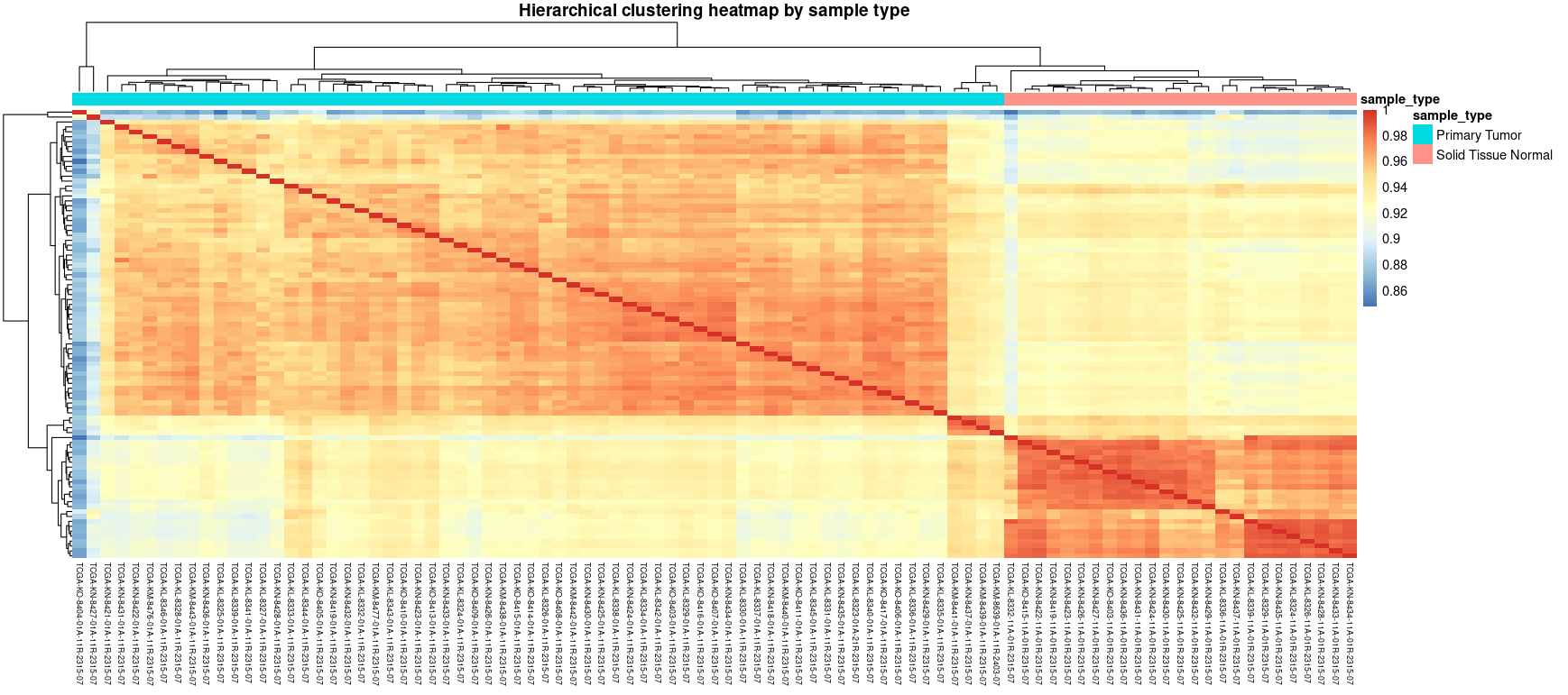
This heatmap shows the Pearson correlation between all samples after variance-stabilizing transformation (VST). Hierarchical clustering reveals clear separation between tumor and normal samples, which is an indicator of consistent expression profiles within each group and successful normalization. Use this plot to check for potential outliers, mislabeled samples or unexpected batch effects.
# Perform PCA to assess sample clustering
plotPCA(vsd, intgroup = "sample_type") +
  ggtitle("PCA plot: Tumor vs Normal samples") +
  theme(plot.title = element_text(hjust = 0.5))

plotPCA(vsd, intgroup = c("sample_type", "gender")) +
  ggtitle("PCA plot: Tumor vs Normal samples (with gender)") +
  theme(plot.title = element_text(hjust = 0.5))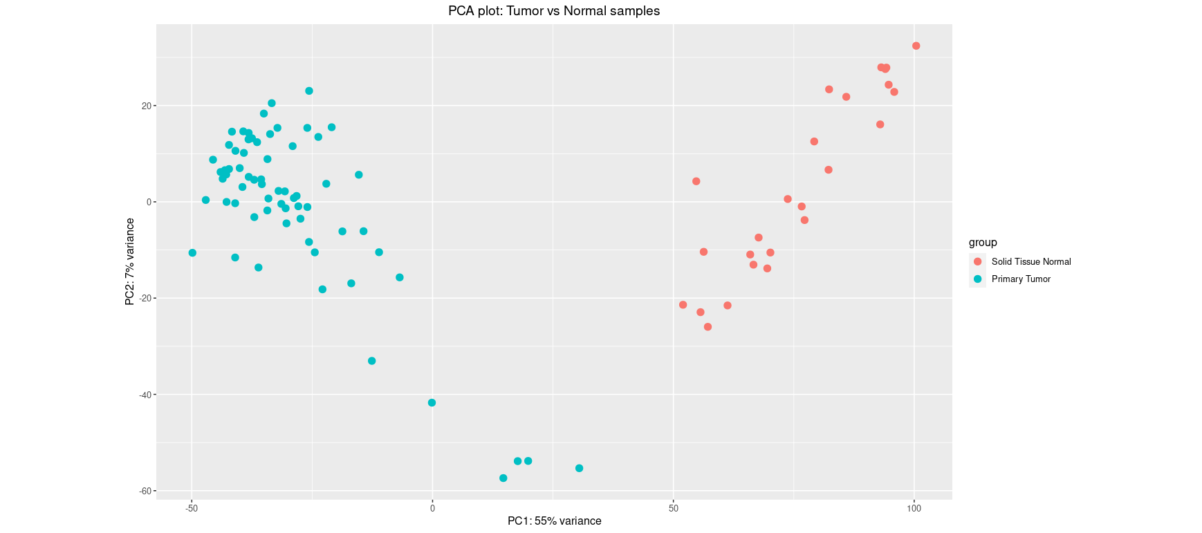
This PCA shows clear separation between tumor and normal samples along PC1 (explaining 55% of the variance). Such clustering suggests that the biological condition (tumor vs normal) is the dominant source of variation. It supports the relevance of differential expression analysis.
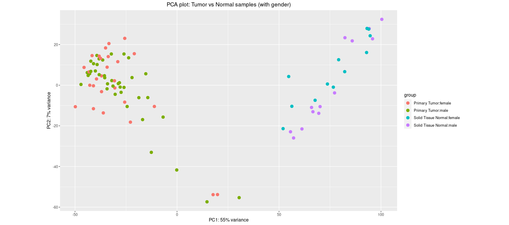
Including gender as a grouping factor helps reveal potential confounding. Here, while sample type still drives most of the separation, some additional structure could be appearing along PC2. If this is the case, gender may explain some expression variance and should be modeled as a covariate in downstream analysis.
# MA-Plot: Inspect differential expression trends
plotMA(res, ylim = c(-8, 8))
title(main = "MA plot", cex.main = 1.5)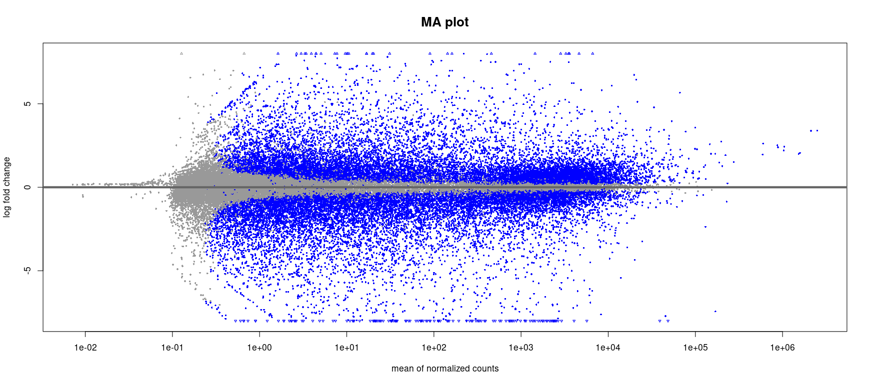
Each dot represents a gene. The x-axis shows the mean normalized count (a proxy for expression level) and the y-axis shows the log2 fold change between tumor and normal samples.
- Genes with low expression tend to have more variability (clouded bottom-left area).
- Blue points indicate genes with adjusted p-value < 0.05.
- This plot highlights many genes with strong up or downregulation (log2FC > |2|), particularly among moderately to highly expressed genes.
# Volcano plot
res <- data.frame(res) %>% mutate(threshold = padj < 0.05) # Generate logical column
res_df <- as.data.frame(res)
res_df$gene <- rownames(res_df)

ggplot(res_df, aes(x = log2FoldChange, y = -log10(padj), color = threshold)) +
  geom_point(alpha = 0.4) +
  theme_minimal() +
  xlab("log2 fold change") +
  ylab("-log10 adjusted p-value") +
  geom_vline(xintercept = c(-1, 1), linetype="dashed", color="red") +
  geom_hline(yintercept = -log10(0.05), linetype="dashed", color="red") +
  ggtitle("Volcano plot") +
  theme(plot.title = element_text(hjust = 0.5, face = "bold")) +
  scale_color_discrete(name = "Adj. p-value < 0.05")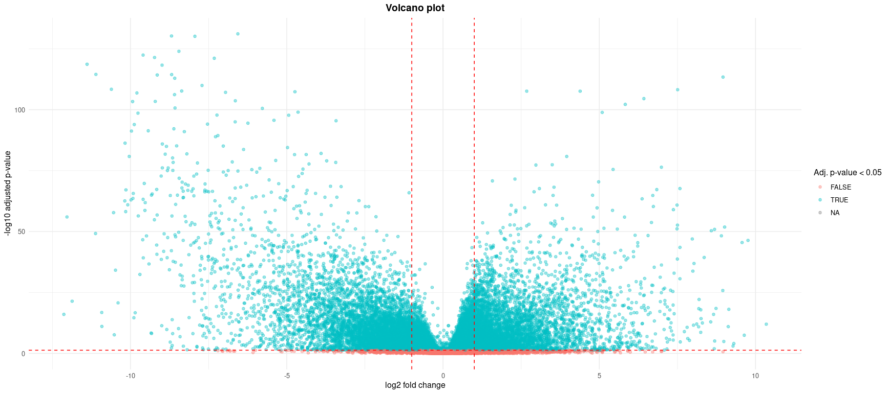
Each point represents a gene, plotted by its log2 fold change (x-axis) and -log10 adjusted p-value (y-axis). Genes with both large expression differences and high statistical significance appear toward the top left or top right.
- Red dashed lines indicate typical cutoffs: |log2FC| > 1 and adjusted p-value < 0.05.
- Blue points (TRUE) denote significantly differentially expressed genes (FDR < 0.05).
- This plot highlights genes of interest for downstream functional analysis or possible validation.
6. Downstream analysis: Functional enrichment
Apply advanced enrichment techniques using clusterProfiler or enrichR to evaluate Gene Ontology (GO) and KEGG pathway enrichments. Ensure conversion to consistent gene identifiers (ENTREZ) is performed. For genes passing significance (adjusted p‑value < 0.05), perform GO enrichment. Convert Ensembl gene IDs (from TCGA) to Entrez IDs using org.Hs.eg.db prior to enrichment.
# Extract significant genes and convert Ensembl IDs to Entrez IDs
sig_genes <- rownames(resOrdered)[!is.na(resOrdered$padj) & resOrdered$padj < 0.05] # adjusted p-value < 0.05
# Remove version numbers from Ensembl IDs
sig_genes_clean <- gsub("\\..*", "", sig_genes)

# Convert Ensembl IDs to Entrez IDs for compatibility with many enrichment tools
converted <- bitr(sig_genes_clean, fromType = "ENSEMBL",
                  toType = "ENTREZID",
                  OrgDb = org.Hs.eg.db)

# Perform GO enrichment analysis (Biological Process)
ego <- enrichGO(gene = converted$ENTREZID,
                OrgDb = org.Hs.eg.db,
                keyType = "ENTREZID",
                ont = "BP",
                pAdjustMethod = "BH",
                pvalueCutoff = 0.05)

# Visualize the top enriched GO terms
dotplot(ego, showCategory = 10) +
  ggtitle("GO enrichment") +
  theme(plot.title = element_text(hjust = 0.5, face = "bold"))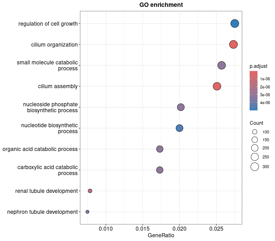
Enriched Gene Ontology (GO) terms are ranked by adjusted p-value and plotted by GeneRatio (number of genes in the input list associated with the term divided by total genes in the term).
- Dot size reflects the number of significant genes associated with each GO term.
- Color gradient shows adjusted p-values, with red indicating stronger statistical significance.
The most enriched biological processes in this dataset include regulation of cell growth, cilium organization and nucleotide biosynthesis, suggesting key pathways altered between tumor and normal tissues.
# Compare enrichment between up/down genes (separate significant genes by direction at an adjusted p-value cutoff of 0.05)
up_genes <- rownames(resOrdered)[!is.na(resOrdered$padj) & resOrdered$padj < 0.05 & resOrdered$log2FoldChange > 0]
down_genes <- rownames(resOrdered)[!is.na(resOrdered$padj) & resOrdered$padj < 0.05 & resOrdered$log2FoldChange < 0]

# Remove version numbers from Ensembl IDs if present
up_genes_clean <- gsub("\\..*", "", up_genes)
down_genes_clean <- gsub("\\..*", "", down_genes)

# ---- GO enrichment using ENSEMBL IDs ----
# This approach assumes Ensembl IDs have been cleaned (no version numbers).
# It works, but might miss some annotations or GO terms due to ID limitations.

# Create a list of gene sets for compareCluster.
# Here, we label the groups to display in the legend.
geneList <- list("Primary Tumor" = up_genes_clean,
                 "Solid Tissue Normal" = down_genes_clean)

# Run compareCluster to perform GO enrichment (Biological Process) on both gene lists
cc <- compareCluster(geneCluster = geneList,
                     fun = "enrichGO",
                     OrgDb = org.Hs.eg.db,
                     keyType = "ENSEMBL",
                     ont = "BP",
                     pAdjustMethod = "BH",
                     pvalueCutoff = 0.05)

dotplot(cc, showCategory = 10) +
  ggtitle("GO enrichment: Tumor vs Normal tissue") +
  theme(plot.title = element_text(hjust = 0.5, face = "bold"),
    axis.text.y = element_text(size = 11)
  )

# ---- Alternative (recommended): Convert to ENTREZ IDs for better coverage ----
# Many GO and pathway databases are more comprehensive when using ENTREZ IDs.
# This improves compatibility and reduces the risk of missing annotations.

up_converted <- bitr(up_genes_clean,
                     fromType = "ENSEMBL",
                     toType = "ENTREZID",
                     OrgDb = org.Hs.eg.db)

down_converted <- bitr(down_genes_clean,
                       fromType = "ENSEMBL",
                       toType = "ENTREZID",
                       OrgDb = org.Hs.eg.db)

# Remove NAs and duplicates
up_entrez <- unique(na.omit(up_converted$ENTREZID))
down_entrez <- unique(na.omit(down_converted$ENTREZID))

# Create gene list
geneList_entrez <- list("Primary Tumor" = up_entrez,
                        "Solid Tissue Normal" = down_entrez)

cc_entrez <- compareCluster(geneCluster = geneList_entrez,
                            fun = "enrichGO",
                            OrgDb = org.Hs.eg.db,
                            keyType = "ENTREZID",
                            ont = "BP",
                            pAdjustMethod = "BH",
                            pvalueCutoff = 0.05)

dotplot(cc_entrez, showCategory = 10) +
  ggtitle("GO enrichment: Tumor vs Normal tissue (ENTREZ IDs)") +
  theme(plot.title = element_text(hjust = 0.5, face = "bold"))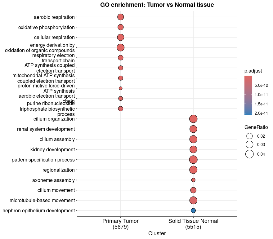
This compareCluster analysis shows enriched Biological Process GO terms for genes upregulated in either Primary Tumor or Solid Tissue Normal samples.
- The x-axis groups gene sets by condition.
- Each dot represents an enriched term, colored by adjusted p-value and sized by gene ratio.
Tumor-upregulated genes are enriched for mitochondrial and energy metabolism processes (aerobic respiration, oxidative phosphorylation) that suggest elevated bioenergetic activity. Normal-upregulated genes show enrichment in developmental and structural terms (renal system development, cilium assembly) that reflect tissue integrity and homeostasis.
These results highlight biological differences between tumor and normal tissues, with tumor cells showing signatures of metabolic reprogramming, a well known hallmark of cancer. Conversely, the enrichment of developmental and structural pathways in normal tissue suggests maintenance of specialized functions lost in tumorigenesis.
This functional context does not only supports the differential expression results but also helps selecting genes/pathways for further validation. You can now explore these gene sets in relation to prognosis or potential therapeutic targets.
🔁 Save your results:
write.csv(resOrdered, "DE_results.csv")
write.csv(normCounts, "Normalized_counts.csv")
This tutorial has walked through a reproducible RNA-seq analysis pipeline using R and Bioconductor, from raw count data through differential expression and functional enrichment. The combination of rigorous statistical modeling and informative visualizations can help you drive biological interpretation. You’re now equipped to extract meaningful insights from bulk transcriptomic datasets. As next steps, consider integrating complementary data types (such as methylation or proteomics) or exploring single-cell RNA-seq for higher resolution.
Session info
# Display session info for reproducibility
sessionInfo()
R version 4.3.3 (2024-02-29)
Platform: x86_64-pc-linux-gnu (64-bit)
Running under: Ubuntu 20.04.6 LTS
attached base packages:
[1] stats4 stats graphics grDevices utils datasets methods base
other attached packages:
[1] pheatmap_1.0.12 ggplot2_3.4.4 org.Hs.eg.db_3.17.0
[4] AnnotationDbi_1.64.0 clusterProfiler_4.8.3 apeglm_1.22.1
[7] sva_3.50.0 BiocParallel_1.34.2 DESeq2_1.40.2
[10] SummarizedExperiment_1.30.2 Biobase_2.60.0 GenomicRanges_1.52.1
[13] IRanges_2.34.1 S4Vectors_0.38.2 BiocGenerics_0.46.0
[16] TCGAbiolinks_2.28.4 tximport_1.28.0